Proportional odds regression
Test multivariate associations when predicting for an ordinal outcome
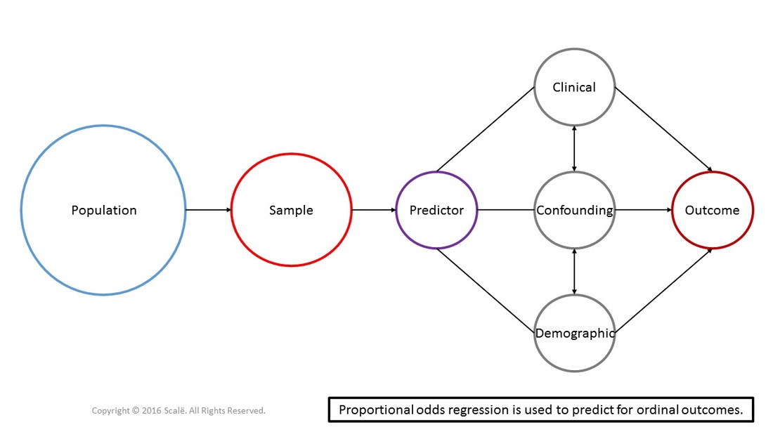
Proportional odds regression is used to predict for ordinal outcomes using predictor, demographic, clinical, and confounding variables. In proportional odds regression, one of the ordinal levels is set as a reference category and all other levels are compared to it. The final odds shows how likely one is to move up on one level in the ordinal outcome. There is a primary assumption of proportional odds regression called the assumption of proportional odds. The odds must stay salient and stable across each level of the ordinal variable for the effect to be valid.
The figure below depicts the use of proportional odds regression. Predictor, clinical, confounding, and demographic variables are being used to predict for an ordinal outcome. Proportional odds regression is a multivariate test that can yield adjusted odds ratios with 95% confidence intervals.
Recode predictor variables to run proportional odds regression in SPSS
SPSS has certain defaults that can complicate the interpretation of statistical findings. When conducting proportional odds regression in SPSS, all categorical predictor variables must be "recoded" in order to properly interpret the SPSS output.
For dichotomous categorical predictor variables, and as per the coding schemes used in Research Engineer, researchers have coded the control group or absence of a variable as "0" and the treatment group or presence of a variable as "1."
In order to correctly interpret the SPSS output, the control group will have to be recoded as "1" and the treatment group will have to be recoded as "0."
For polychotomous categorical predictor variables, the recoding becomes a little bit more complicated, but basic numerical logic will yield the correct answer.
As an example, let's say that there is a polychotomous categorical variable with four levels. Researchers have coded "0" as the control group, "1" as the second group, "2" as the third group, and the fourth and final group as "3."
With the defaults in SPSS, this variable will needed to be recoded with "3" as the control group, "2" as the second group, "1" as the third group, and the fourth and final group as "0."
The steps for conducting a proportional odds regression in SPPS
1. The data is entered in a multivariate fashion.
2. Click Analyze.
3. Drag the cursor over the Regression drop-down menu.
4. Click Ordinal.
5. Click on the ordinal outcome to highlight it.
6. Click on the arrow to move the variable into the Dependent: box.
7. Click on a categorical predictor variable to highlight it.
8. Click on the arrow to move the variable into the Factor(s) box.
9. Repeat Steps 7 and 8 until all of the categorical predictor variables are in the Factor(s) box.
10. Click on a continuous predictor variable to highlight it.
11. Click on the arrow to move the variable into the Covariate(s): box.
12. Click on the Output button.
13. In the Display table, click on the Test of parallel lines box to select it.
14. Click Continue.
15. Click OK.
The steps for interpreting the SPSS output for a proportional odds regression
1. Look in the Model Fitting Information table, under the Sig. column. This is the p-value that is interpreted.
If the p-value is LESS THAN .05, then the model fits the data and is significant. Researchers can proceed with the interpretation.
If the p-value is MORE THAN .05, then the model does not fit the data and is not significant.
2. Look in the Parameter Estimates table, under the Sig. column. These are the p-values that is interpreted.
If the p-value is LESS THAN .05, then for every one unit increase in the variable, the log odds of moving into a higher level of the ordinal outcome increases (or decreases) that much.
If the p-value is MORE THAN .05, then the variable is not significant.
Users may have noticed that instead of using "odds," "odds ratio," "more likely, or "less likely" above, I used the terms "log odds" and "increases" or "decreases." The reason for this is that SPSS does not generate the adjusted odds ratios with 95% confidence intervals.
So, what you will have to do is EXPONENTIATE these values in order to get the adjusted odds ratios with 95% CIs. The easiest way to generate these values is to write down the values in the Estimate, Lower Bound, and Upper bound columns for the significant predictor variables in your model, and then download the Exponentiate spreadsheet below.
The adjusted odds ratios with 95% confidence intervals are the appropriate statistics to report for this type of analysis. Non-significant associations should be reported as well.
Residuals and proportional odds regression
At this point, researchers need to construct and interpret several plots of the raw and standardized residuals to fully assess model fit. Residuals can be thought of as the error associated with predicting or estimating outcomes using predictor variables. Residual analysis is extremely important for meeting the linearity, normality, and homogeneity of variance assumptions of proportional odds regression.
However, it is going to be a tedious process. Take the number of levels of your ordinal outcome variable, subtract one, and that is the number of times the analysis will have to be performed.
To make this a simple example, let's say that reserachers have found a significant main effect using a 5-point Likert scale variable with the reference category outcome level codified as "0," with the next level of the outcome = 1, the next level = 2, the next level = 3, and the last level = 4. Researchers will have to perform the analyses four times to fully assess model fit.
Step 1: Perform a binary logistic regression analysis with reference category outcome = 0 and the next level of the outcome = 1.
With the aforementioned coding scheme:
1. Click Data.
2. Click Select Cases.
3. In the Select table, click on the If condition is satisfied marker to select it.
4. Click on the If button.
5. Click on the polychotomous categorical outcome variable to highlight it.
6. Click on the arrow to move it into the box.
7. Click the <= button.
8. Type the number, "1"
9. Click Continue.
10. Click OK.
Step 2: Go to Data View. Researchers will see that only the observations with a "0" or "1" as an outcome are highlighted. Perform a logistic regression analysis on this data. Click on the button to learn how to conduct a logistic regression analysis:
Step 3: Perform the residual analysis for the logistic regression in SPSS:
1. There are three new variables that have been created.
The first is the predicted probability of that observation and is given the variable name of PRE_1.
The second variable contains the raw residuals (the difference between the observed and predicted probabilities of the model) and is given the variable name of RES_1.
The third variable has standardized residuals based on the raw residuals in the second variable and will be given the variable name of as ZRE_1.
2. Click Graphs.
3. Drag the cursor over the Legacy Dialogs drop-down menu.
4. Click Scatter/Dot.
5. Click Simple Scatter to select it.
6. Click Define.
7. Click on the RES_1 or raw residual variable to highlight it.
8. Click on the arrow to move the variable into the Y Axis: box.
9. Click on the PRE_1 or predicted probability variable to highlight it.
10. Click on the arrow to move the variable into the X Axis: box.
11. Click OK.
Here is how to interpret the scatterplot:
1. If the points along the scatterplot are symmetric both above and below a straight line, with observations being equally spaced out along the line, then the assumption of linearity can be assumed. Interpretation of these types of scatterplot graphs allows for some subjectivity in regards to symmetry and spread along the line.
If there are significantly larger residuals and wider dispersal of observations along the line, then linearity cannot be assumed.
Outliers and proportional odds regression
Step 4: Normality and equal variance assumptions apply to proportional odds regression analyses. Here is how to assess for outliers:
1. Click Analyze.
2. Drag the cursor over the Descriptive Statistics drop-down menu.
3. Click Frequencies.
4. Click on the ZRE_1 or standardized residuals variable to highlight it.
5. Click on the arrow to move the variable into the Variable(s): box.
6. Click OK.
2. Drag the cursor over the Descriptive Statistics drop-down menu.
3. Click Frequencies.
4. Click on the ZRE_1 or standardized residuals variable to highlight it.
5. Click on the arrow to move the variable into the Variable(s): box.
6. Click OK.
Here is how to interpret the SPSS output:
1. Look in the Normalized residual table, under the first column. (It has the word "Valid" in it).
2. Scroll through the entirety of the table.
3. If there are values that are above an absolute value of 2.0, then there are outliers.
1. Look in the Normalized residual table, under the first column. (It has the word "Valid" in it).
2. Scroll through the entirety of the table.
3. If there are values that are above an absolute value of 2.0, then there are outliers.
Further analyses and proportional odds regression
Step 5: Conduct this exact same analysis, but with the reference category as "0" and the next level of the ordinal variable as the outcome = 2.
Here are the steps for switching the levels of the outcome that are being modeled:
1 Click Data.
2. Click Select Cases.
3. In the Select table, click on the If condition is satisfied marker to select it.
4. Click on the If button.
5. Clear out the box where the formula goes on the right hand side of the window.
6. Type this: ("Outcome name" = 0) OR ("Outcome name" = 2)
Where "Outcome name" means the variable's name.
7. Click Continue.
8. Click OK.
Step 6: Go to Data View. Researchers will see that only the observations with a "0" or "2" as an outcome are highlighted. Perform a logistic regression analysis on this data AND all of the subsequent residual analyses. Repeat the individual logistic regression analyses until all of the levels of the ordinal outcome variable have been compared to the reference category. If all of the respective models meet the assumptions of linearity, normality, and homogeneity of variance, the overall proportional odds model is assumed to fit the data.
Proportional odds assumption
As you create these necessary models to assess model fit, researchers can assess meeting a specific and unique statistical assumption of this regression analysis, the proportional odds assumption. This assumption assesses if the odds of the outcome occurring is similar across values of the ordinal variable. If the odds ratios are similar across models at different cut-points and to the cumulative odds ratio, then this assumption is assumed to be met.
Click on the Download Database and Download Data Dictionary buttons for a configured database and data dictionary for proportional odds regression. Click on the Validation of Statistical Findings button to learn more about bootstrap, split-group, and jack-knife validation methods.

Hire A Statistician
DO YOU NEED TO HIRE A STATISTICIAN?
Eric Heidel, Ph.D., PStat will provide you with statistical consultation services for your research project at $100/hour. Secure checkout is available with Stripe, Venmo, Zelle, or PayPal.
- Statistical Analysis on any kind of project
- Dissertation and Thesis Projects
- DNP Capstone Projects
- Clinical Trials
- Analysis of Survey Data