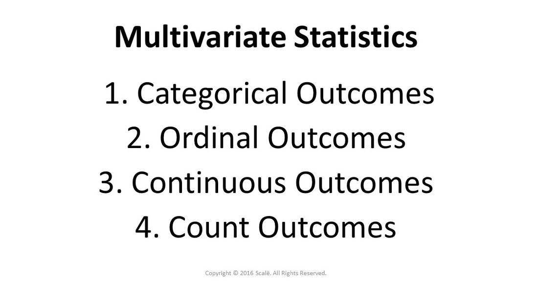
Multivariate statistics
Multivariate statistics account for confounding variables and predict for outcomes
Multivariate statistics are used to account for confounding effects, account for more variance in an outcome, and predict for outcomes. Multivariate statistics allows for associations and effects between predictor and outcome variables to be adjusted for by demographic, clinical, and prognostic variables (simultaneous regression). Multivariate statistics further represent "reality" in that very few, if any, associations and effects are bivariate in nature. Multivariate statistics can further be used to choose the best set of predictors for predicting outcomes (stepwise regression). Finally, multivariate statistics can be used to test theoretical, conceptual, or physiological frameworks (hierarchical regression).
Before running any multivariate statistics, there are several tasks to complete in regards to structuring the data and the meeting of certain statistical assumptions. Let's get started!
Before running any multivariate statistics, there are several tasks to complete in regards to structuring the data and the meeting of certain statistical assumptions. Let's get started!
Preparing data for multivariate analysis
1. Continuous predictor variables must be normally distributed and have equal variance across the outcome. Run skewness and kurtosis statistics to assess this assumption. Equal variance or homoscedasticity will be assessed later.
2. Dichotomous or polychotomous categorical predictor variables must be coded into mutually exclusive categorical variables. Rese archersmust also set a reference group to which other levels of the categorical variable will be compared. For ease of analysis and interpretation, always code the reference category as "0."
For example, researchers would code NOT having a characteristic or outcome as a "0" and HAVING a characteristic or outcome as a "1" for dichotomous variables.
When it comes to polychotomous categorical variables (3 or more independent levels), a little bit more complexity is added to the analysis. Researchers will need to create a new set of variables to account for the multiple levels of the categorical predictor. The formula for the number of variables need is, (The number of levels of your categorical predictor variable - 1). So, if researchers have seven levels or groups of an independent categorical predictor variable, they will have to create six mutually exclusive between-subjects variables to account for them. If researchers have six levels, they would create five variables. If there were five levels, they would create four variables, and so on.
The reason that researchers create one less variable than the number of levels of the categorical predictor variable is that the reference category is created by default with the non-existence, non-exposure, or lack of possessing the characteristic of all the other levels combined. If six mutually exclusive between-subjects variables are codified as 0 = NOT having the characteristic and 1 = HAVING the characteristic, then there is a chance that someone in the sample may not possess ANY of those six characteristics, and thus would be in the reference category, codified as six "0's" across the six mutually exclusive between-subjects variables.
This complexity can be readily ascertainable with a basic example of using eye color as a predictor in a study focused on eye shadow. There are blue eyes, green eyes, and brown eyes being rated. Researchers would create two mutually exclusive between-subjects variables to account for this in a multiple regression analysis (3 groups - 1 = 2 variables). Let's say blue eyes is the reference group. Researchers would code the "green eyes" variable as 0 = DOES NOT have green eyes and 1 = DOES have green eyes. Then, the "brown eyes" variable would be codified as 0 = DOES NOT have brown eyes and 1 = DOES have brown eyes. Lastly, the reference group, "blue eyes," exists by default as a rating of 0 for both "green eyes" and "brown eyes."
NOTE: Step 2 only applies if researchers are using polychotomous variables in multiple regression. SPSS creates these categories automatically through the point-and-click interface when conducting all the other forms of multivariate analysis.
3. Run scatterplots between the continuous predictor variables and the outcome. If there is a non-linear relationship, according to the scatterplots, consider running a logarithmic transformation on the predictor variable. All predictor variables must have some sort of linear relationship with the outcome.
4. Researchers must run bivariate correlations among all of the predictor variables entered into a model. This is done to ensure that the model does not possess multicollinearlity. This is the phenomenon where predictor variables are highly correlated to each other, or essentially, measuring the same thing TWICE in a model. This can artificially inflate or deflate the t-test values associated with the model.
Multicollinearity is assessed statistically using two different methods: Tolerance and the variance inflation factor (VIF). Smaller tolerance values (below .60) denote the presence of multicollinearity. VIF values above 2.5 also suggest the presence of multicollinearity.
If any pair of variables correlates at above .80, consider deleting one of the variables from the model or combining them in some fashion.
5. Do not include any spurious variables or variables that have more than 20% missing data in their distribution. Include variables that exist in the literature and exist within a theoretical, conceptual, or physiological framework together. Include only confounding variables yielded from the literature. To achieve enough statistical power, a minimum of 20 observations of the outcome per variable should be included in the model.
Scale of measurement for the outcome in multivariate statistics
The outcome represents numerical designations or categorical values that describe events or group membership.
The outcome variable is measured using an ordered numerical continuum, such as a Likert scale.
The outcome variable is an actual number that provides both a measure of distance and magnitude due to having a "true zero."
The outcome variable is the actual number of times an event occurs.
There are multiple continuous outcomes being compared across independent groups.
Multivariate statistics and regression
Step-by-step methods for conducting and interpreting logistic regression, multinomial logistic regression, Cox regression, proportional odds regression, multiple regression, Poisson regression, and negative binomial regression in SPSS.*
Learn more about the importance of assessing model fit in regression models.
Learn more about testing for homoscedasticity in regression models.
Learn more about the linearity assumption in regression models.
Hire A Statistician
DO YOU NEED TO HIRE A STATISTICIAN?
Eric Heidel, Ph.D., PStat will provide you with statistical consultation services for your research project at $100/hour. Secure checkout is available with Stripe, Venmo, Zelle, or PayPal.
- Statistical Analysis on any kind of project
- Dissertation and Thesis Projects
- DNP Capstone Projects
- Clinical Trials
- Analysis of Survey Data
*SPSS Version 21 (Armonk, NY: IBM Corp.)

