Random-effects ANOVA
Test interactions between multiple observations of outcomes
Random-effects ANOVA is used to answer research questions where the variance across observations and within-subjects effects can be assessed across different levels of categorical variables. With random-effects ANOVA, there are demographic, prognostic, and clinical variables that confound and mitigate associations between predictor and outcome variables. Random-effects ANOVA allows you to answer these more complex research questions, and thus, generate evidence that is more indicative of the outcome as it truly exists in the population of interest. The random-effects ANOVA focuses on how "random" observations of an outcome vary across two or more within-subjects variables.
For example, let's say researchers are interested in the effects of a new therapy for people with social anxiety and the number of sick days they use yearly. A validated measure of social anxiety would be administered to study participants to assess their baseline level of social anxiety and the number of sick days they had utilized at baseline. Then, at six months after participating in the new therapy regimen, a second observation of social anxiety and sick days used would be taken. The same would be repeated at 12 months. Therefore, you can assess how these two "random" effects change and interact with each other across time or within-subjects.
Researchers are essentially answering three research questions with one analysis: Was there a significant main effect across time for the first "random" variable? Was there a significant main effect across time for the second "random" variable? Do the two "random" variables adjust the outcome variable in a significant fashion?
The marginal means and errors for each level of the interaction should be presented. Significant main effects must be further tested in a post hoc fashion to assess where amongst the levels of the interaction the significance exists and when there are more than two "random" observations of the outcome.
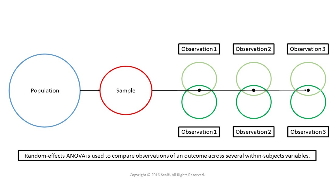
The figure below depicts the use of random-effects ANOVA. There is only one group being observed. Observations of two difference within-subjects variables are being taken at multiple times moving forward. Random-effects ANOVA yields marginal means and standard errors.
The steps for conducting a random-effects ANOVA
1. The data is entered in a within-subjects fashion.
2. Click Analyze.
3. Drag the cursor over the General Linear Model drop-down menu.
4. Click Repeated-Measures.
5. Type the name of the first "random" or within-subjects variable into the Within-Subject Factor Name: box.
6. Type the number of observations of the outcome into the Number of Levels: box.
7. Click the Add button to move the variable into the box.
8. Type of the name of the second "random" or within-subjects variable into the Within-Subject Factor Name: box.
9. Type the number of observations of the outcome into the Number of Levels: box.
10. Click the Add button to move the variable into the box.
11. Click Define.
12. Click on the first observation of the first "random" or within-subjects variable to highlight it.
13. Click on the arrow to move the variable into the (1,1) row of the Within-Subjects Variables (Variable 1 name, Variable 2 name): box.
14. Click on the second observation of the first "random" or within-subjects variable to highlight it.
15. Click on the arrow to move the variable into the (1,2) row of the Within-Subjects Variables (Variable 1 name, Variable 2 name): box.
16. Click on the first observation of the second "random" or within-subjects variable to highlight it.
17. Click on the arrow to move the variable into the (2,1) row of the Within-Subjects Variables (Variable 1 name, Variable 2 name): box.
18. Click on the second observation of the second "random" or within-subjects variable to highlight it.
19. Click on the arrow to move the variable into the (2,2) row of the Within-Subjects Variables (Variable 1 name, Variable 2 name): box.
20. Click on the Plots button.
21. Click on the first "random" or within-subjects variable to highlight it.
22. Click on the arrow to move the variable into the Separate Lines: box.
23. Click on the second "random" or within-subjects variable to highlight it.
24. Click on the arrow to move the variable into the Horizontal Axis: box.
25. Click on the Add button.
26. Click Continue.
27. Click on the Options button.
28. In the Factor(s) and Factor Interactions: table, click on the first "random" or within-subjects variable to highlight it.
29. Click on the arrow to move the variable into the Display Means for: box.
30. Repeat Steps 26 and 27 until all of the "random" or within-subjects variables and the interaction are moved into the Display Means for: box.
31. Click on the Compare main effects box to select it.
32. In the Display table, click on the Descriptive statistics, Estimates of effect size, and Observed power boxes to select them.
33. Click Continue.
34. Click OK.
The steps for interpreting the SPSS output for a random-effects ANOVA
1. Scroll down to the Tests of Within-Subjects Effects table and look in the Sig. column. These are the p-values that are interpreted. Interpret the Greenhouse-Geisser corrected value.
2. Look at the value for the first "random" or within-subjects variable.
If the p-value is LESS THAN .05, then researchers have evidence of a statistically significant change across time or within-subjects for that variable.
If the p-value is MORE THAN .05, then researchers do NOT have evidence of a statistically significant change across time or within-subjects.
3. Look at the p-value for the second "random" or within-subjects variable.
If the p-value is LESS THAN .05, then researchers have evidence of a statistically significant change across time or within-subjects for that variable.
If the p-value is MORE THAN .05, then researchers do NOT have evidence of a statistically significant change across time or within-subjects for that variable.
4. Look at the p-value for the first*second "random" effects interaction.
If the p-value is LESS THAN .05, then researchers have evidence of a statistically significant change across time or within-subjects for the interaction.
If the p-value is MORE THAN .05, then researchers do NOT have evidence of a statistically significant change across time or within-subjects for the interaction.
5. If researchers have a significant main or interaction effect, scroll down to the Estimated Marginal Means section of the output.
6. For each "random" level or within-subjects variable, look in the Estimates table for the means and standard errors for each observation.
7. For each "random" level or within-subjects variable, look in the Pairwise Comparisons table under the Sig. column. These are the p-values associated with the post hoc comparisons.
If the p-value is LESS THAN .05, then researchers have evidence of a statistically significant change across time or within-subjects for that variable.
If the p-value is MORE THAN .05, then researchers do NOT have evidence of a statistically significant change across time or within-subjects for that variable.
8. Scroll down to the table with the first*second "random" variables names as the title.
9. These are the marginal means and standard deviations for each level of the interaction between the "random" variables.
10. The graph provides a visual aid at understanding the main and interaction effects.
Click on the Download Database and Download Data Dictionary buttons for a configured database and data dictionary for random-effects ANOVA. Click on the Validation of Statistical Findings button to learn more about bootstrap, split-group, and jack-knife validation methods.

Hire A Statistician
DO YOU NEED TO HIRE A STATISTICIAN?
Eric Heidel, Ph.D., PStat will provide you with statistical consultation services for your research project at $100/hour. Secure checkout is available with Stripe, Venmo, Zelle, or PayPal.
- Statistical Analysis on any kind of project
- Dissertation and Thesis Projects
- DNP Capstone Projects
- Clinical Trials
- Analysis of Survey Data