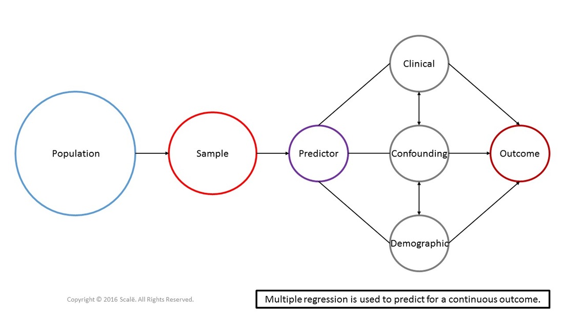
Multiple regression is used to predictor for continuous outcomes. In multiple regression, it is hypothesized that a series of predictor, demographic, clinical, and confounding variables have some sort of association with the outcome. The continuous outcome in multiple regression needs to be normally distributed. The predictor, demographic, clinical, and confounding variables can be entered into a simultaneous model (all together at the same time), in a stepwise model (where an algorithm picks the best group of variables that account for the most variance in the outcome), or in a hierarchical model (a theoretical framework is used to choose the order or entry into a model). Multiple regression yields an algorithm that can predict for a continuous outcome.
The figure below depicts the use of multiple regression (simultaneous model). Predictor, clinical, confounding, and demographic variables are being used to predict for a continuous outcome that is normally distributed. Multiple regression is a multivariate test that yields beta weights, standard errors, and a measure of observed variance.

1. The data is entered in a multivariate fashion.
2. Click Analyze.
3. Drag the cursor over the Regression drop-down menu.
4. Click Linear.
5. Click on the continuous outcome variable to highlight it.
6. Click on the arrow to move the variable into the Dependent: box.
7. Click on the first predictor variable to highlight it.
8. Click on the arrow to move the variable into the Independent(s): box.
9. Repeat Steps 7 and 8 until all of the predictor variables are in the Independent(s): box.
10. Click on the Statistics button.
11. Click on the R squared change, Collinearity diagnostics, Durbin-Watson, and Casewise diagnostics boxes to select them.
12. Click on the Plots button.
13. Click on the DEPENDNT variable to highlight it.
14. Click on the arrow to move the variable into the X: box.
15. Click on the *ZRESID variable to highlight it.
16. Click on the arrow to move the variable into the Y: box.
17. In the Standardized Residual Plots table, click on the Histogram and Normal probability plot boxes to select them.
18. Click Continue.
19. Click OK.
1. Look in the Model Summary table, under the R Square and the Sig. F Change columns. These are the values that are interpreted.
The R Square value is the amount of variance in the outcome that is accounted for by the predictor variables you have used.
If the p-value is LESS THAN .05, the model has accounted for a statistically significant amount of variance in the outcome.
If the p-value is MORE THAN .05, the model has not accounted for a significant amount of the outcome.
2. Look in the Coefficients table, under the B, Std. Error, Beta, Sig., and Tolerance columns.
The B column contains the unstandardized beta coefficients that depict the magnitude and direction of the effect on the outcome variable.
The Std. Error contains the error values associated with the unstandardized beta coefficients.
The Beta column presents unstandardized beta coefficients for each predictor variable.
The Sig. column shows the p-value associated with each predictor variable.
If a p-value is LESS THAN .05, then that variable has a significant association with the outcome variable.
If a p-value is MORE THAN .05, then that variable does not have a significant association with the outcome variable.
The Tolerance column presents values related to assessing multicollinearity among the predictor variables.
If any of the Tolerance values are BELOW .75, consider creating a new variable or deleting one of the predictor variables.
At this point, researchers need to construct and interpret several plots of the raw and standardized residuals to fully assess the fit of your model. Residuals can be thought of as the error associated with predicting or estimating outcomes using predictor variables. Residual analysis is extremely important for meeting the linearity, normality, and homogeneity of variance assumptions of multiple regression.
Scroll down the bottom of the SPSS output to the Scatterplot. If the plot is linear, then researchers can assume linearity.
Normality and equal variance assumptions apply to multiple regression analyses.
Look at the P-P Plot of Regression Standardized Residual graph. If there are not significant deviations of residuals from the line and the line is not curved, then normality and homogeneity of variance can be assumed.
Click on the Download Database and Download Data Dictionary buttons for a configured database and data dictionary for multiple regression. Click on the Validation of Statistical Findings button to learn more about bootstrap, split-group, and jack-knife validation methods.