The mixed-effects ANOVA compares how a continuous outcome changes across time (random effects) between independent groups or levels (fixed effects) of a categorical predictor variable.
For example, let's say researchers are interested in the change of number of hours of reality TV watched (continuous outcome) between men and women (fixed effect) as the college football season leads into the college basketball season (random effect). Gender is a "fixed" effect in that each participant is represented in one of the independent groups or levels of the "factor." Observations of number of hours of reality TV watched (let's say at the beginning of the college football season, then, at the beginning of the basketball season, and finally, at the end of March) is the "random" effect. Therefore, you can assess how the number of hours watched changes across time AND between different groups. You will be able to show evidence of how men change in number of hours watched from late August all the way until March of the next year and compare that level of change to how women change in number of hours watched along that same time frame.
The marginal means and errors for each level of the interaction should be presented in a mixed-effects ANOVA. Significant main effects must be further tested in a post hoc fashion to assess where among the levels of the interaction the significance exists and when the "fixed" or "random" effects are polychotomous (more than two "fixed" levels or observation of a variable) in the mixed-effects ANOVA analysis.
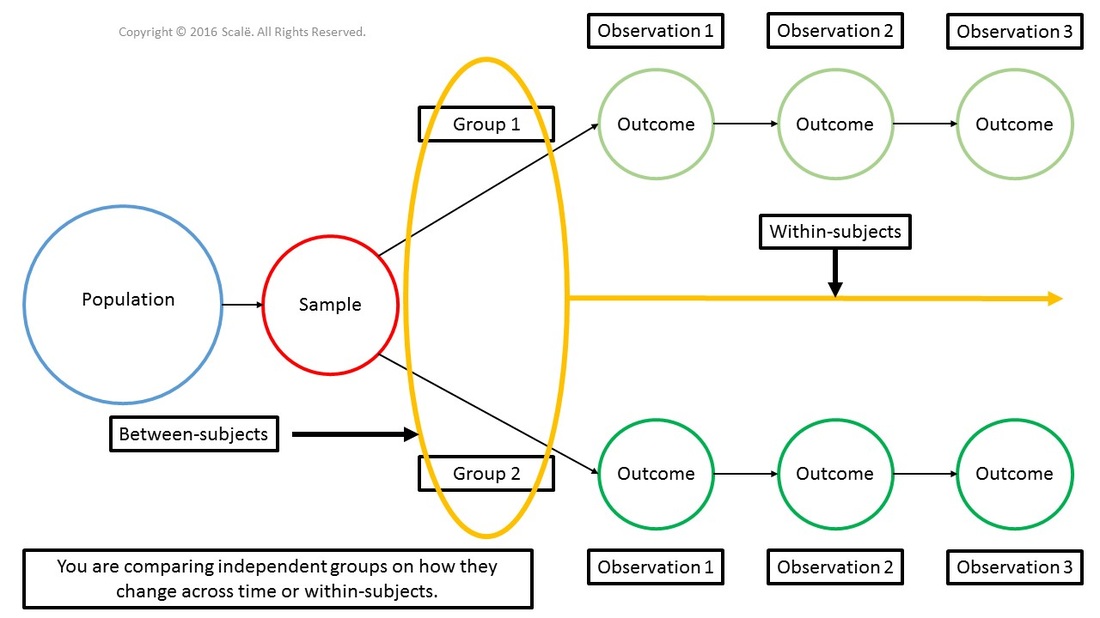
The figure below depicts the use of mixed-effects ANOVA. There are two independent groups being compared on how they change across time in terms of an outcome taken at three time points.

1. The data is entered using a mixed method.
2. Click Analyze.
3. Drag the cursor over the General Linear Model drop-down menu.
4. Click on Repeated Measures.
5. In the Within-Subject Factor Name: box, type the name of the outcome that is being observed multiple times or within-subjects.
6. In the Number of Levels: box, type the number of observations of the outcome are being assessed. (Pretest -- Posttest = 2, Pretest -- Posttest -- Maintenance = 3, and so on)
7. Click the Add button.
8. Click Define.
9. Click on the first observation of the continuous outcome to highlight it.
10. Click on the arrow to move the variable into the Within-Subjects Variables (Outcome name): box.
11. Repeat Steps 8 and 9 until all the observations of the outcome are in the Within-Subjects Variables (Outcome name): box.
12. Click on the "fixed" effect variable (groups, categorical variable) to highlight it.
13. Click on the arrow to move the variable into the Between-Subjects Factor(s): box.
14. Click on the Plots button.
15. Click on the "fixed" effect variable to highlight it.
16. Click on the arrow to move the variable into the Separate Lines: box.
17. Click on the "random" effect variable to highlight it.
18. Click on the arrow to move the variable into the Horizontal Axis: box.
19. Click the Add button.
20. Click Continue.
21. Click the Options button.
22. Look in the Estimated Marginal Means table, in the Factor(s) and Factor Interactions: box. Click on the "fixed" effect variable to highlight it.
23. Click on the arrow to move the variable into the Display Means for: box.
24. Repeat Steps 21 and 22 until all of the "fixed" and "random" effects are in the Display Means for: box.
25. Click on the Compare main effects box to select it.
26. Look in the Display table, click on the Descriptive statistics, Estimates of effect size, Observed power, and Homogeneity tests boxes to select them.
27. Click Continue.
28. Click OK.
1. Look in the Box's Test of Equality of Covariance Matrices table. If the p-value in the Sig. row is MORE THAN .05, continue with the analysis. If the p-value is LESS THAN .05, reassess the observations for outliers and rerun the analysis.
2. Look in the Mauchly's Test of Sphericity table, under the Sig. column.
If this p-value is MORE THAN .05, researchers will interpret the p-values in the Multivariate Tests table.
If this p-value is LESS THAN .05, researchers will interpret a Greenhouse-Geisser corrected analysis in the Tests of Within-Subjects Effects table.
3. If the p-value was MORE THAN .05 in the table above, look in the Multivariate Tests table of the output, under the Sig. column. These are the p-values that are interpreted for the change across time for all study participants and the interaction between the "fixed" and "random" effects.
If a p-value is LESS THAN .05, then researchers have evidence of a significant main effect.
If a p-value is MORE THAN .05, then researchers do not have evidence of a significant main effect.
4. If the p-value was LESS THAN .05 (which happens more times than not), look in the Tests of Within-Subjects Effects table, under the Sig. column. Interpret the p-values for the change across time for all study participants and the interaction between the "fixed" and "random" effects that are in the Greenhouse-Geisser row.
If the p-value is LESS THAN .05, then researchers have evidence of a significant main effect.
If the p-value is MORE THAN .05, then researchers do not have evidence of a significant main effect.
5. If researchers found a significant main effect, look in the Tests of Within-Subjects Contrasts table, under the Sig. column. The p-values in this column are focused on testing linear and quadratic effects. A linear effect travels in one direction, either "up" or "down." A quadratic effect is an effect that goes "up" and then goes "down" or it will go "down" and then go back "up."
An example of this would be the half-life of a medication. As soon as the pill is ingested, the level of the medication in the bloodstream will significantly increase, but over time, the amount of the drug will dissipate as the body metabolizes the medicine.
A p-value of LESS THAN .05 denotes either a significant linear or quadratic effect.
A p-value of MORE THAN .05 means there was not a significant linear or quadratic effect.
6. If researchers found a significant main effect, scroll down to the Estimated Marginal Means section of the output. The means for both "fixed" and "random" effects are presented first. These p-values are testing the entire sample, without taking the other variable into consideration. For the "fixed" effect, look in the Pairwise Comparisons table, under the Sig. column. These are the p-values associated with comparing the independent groups or levels of the categorical "fixed" effect. For the "random" effect, look at the Pairwise Comparisons table, under the Sig. column. These are the p-values associated with the "random" effects or observations of the outcome. Any p-value that is LESS THAN .05 means there is evidence of a significant difference between-groups or within-subjects. A p-value that is MORE THAN .05 means that there is not a significant difference between-groups or within-subjects.
7. Based on having a significant interaction effect, the "fixed"*"random" table presents the marginal means and standard errors associated with the interaction.
8. Lastly, there is a graph that serves a visual aid for understanding the p-values.
Click on the Download Database and Download Data Dictionary buttons for a configured database and data dictionary for mixed-effects ANOVA. Click on the Validation of Statistical Findings button to learn more about bootstrap, split-group, and jack-knife validation methods.