Greenhouse-Geisser
Correct for violating the assumption of sphericity with repeated-measures ANOVA
The Greenhouse-Geisser is used to assess the change in a continuous outcome with three or more observations across time or within-subjects. In most cases, the assumption of sphericity is violated for this type of within-subjects analysis and the Greenhouse-Geisser correction is robust to the violation. Means and standard deviations should be reported for each observation of the outcome with Greenhouse-Geisser corrections.
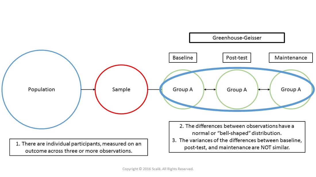
The figure below depicts the use of a Greenhouse-Geisser correction. There is only one group being observed at three or more within-subjects observations or time points. The assumption of normality of difference scores has been met, but the assumption of sphericity has been violated. When the assumption of sphericity is violated with repeated-measures ANOVA, then the Greenhouse-Geisser correction is used.
The steps for conducting a Greenhouse-Geisser correction in SPSS
1. The data is entered in a within-subjects fashion.
2. Click Analyze.
3. Drag the cursor over the General Linear Model drop-down menu.
4. Click Repeated Measures.
5. Type the number of observations of the continuous outcome that are being collected into the Number of Levels: box.
6. In the Within-Subject Factor Name: box, give the outcome variable a name. Example: "Outcome"
7. Click the Add button.
8. Click the Define button.
9. Click on the first observation of the continuous outcome.
10. Click on the arrow to move the outcome variable into the Within-Subjects Variables: box.
11. Click on the second observation of the continuous outcome.
12. Click on the arrow to move the outcome variable into the Within-Subjects Variables: box.
13. Click on the third observation of the continuous outcome.
14. Click on the arrow to move the outcome variable into the Within-Subjects Variables: box.
15. Click on the Options button.
16. Click on the outcome variable to highlight it.
17. Click on the arrow to move the outcome into the Display Means for: box.
18. Click on the Compare main effects box to select it.
19. Click on the Descriptive statistics box to select it.
20. Click on the Estimates of effect size box to select it.
21. Click on the Observed power box to select it.
22. Click Continue.
23. Click on the Plots button.
24. Click on the outcome variable to highlight it.
25. Click on the arrow to move the outcome into the Horizontal Axis: box.
26. Click the Add button.
27. Click Continue.
28. Click OK.
The steps for interpreting the SPSS output for Greenhouse-Geisser
1. In the Tests of Within-Subjects Effects table, look under the Sig. column for the Greenhouse-Geisser row value. This is the p-value that is interpreted. In the Partial Eta Squared column, there is a measure of effect size for the analysis. Under Observed Power, there is the achieved power yielded from conducting the study.
If the p-value is LESS THAN .05, then researchers have evidence of a statistically significant main effect amongst the observations of the outcome or within-subjects.
If the p-value is MORE THAN .05, then researchers have evidence of that a significant main effect does NOT exist amongst the observations of the outcome or within-subjects.
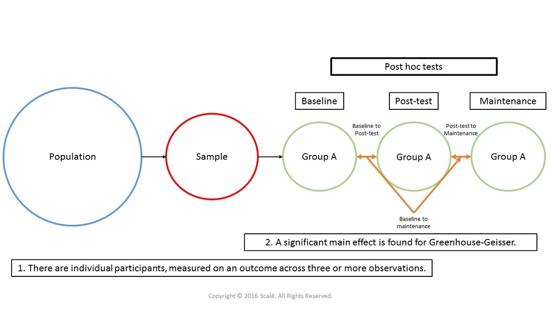
If a significant main effect is found, then pairwise comparisons should be used in a post hoc fashion to establish within-subjects differences. The figure below depicts the use of post hoc tests when a significant main effect is found for a Greenhouse-Geisser correction.
The steps for interpreting the SPSS output for post hoc tests
In the Pairwise Comparisons table, look under the Sig. column.
If the p-value is LESS THAN .05, then there is a statistically significant difference between the two observations identified in the (I) Outcome and (J) Outcome columns.
If the p-value is MORE THAN .05, then there is NOT a statistically significant difference between the two observations identified in the (I) Outcome and (J) Outcome columns.
Interpretation of the p-values must be done within the context of the means and standard deviations. For example, researchers would say, there was a significant main effect for the outcome, p < .05. Post hoc comparisons were conducted. There were significant differences between "Observation 1" (mean and standard deviation), "Observation 2" (mean and standard deviation), and "Observation 3" (mean and standard deviation), p = .01.
It is HIGHLY IMPORTANT to interpret the p-values within the context of the means and standard deviations that are presented in the Descriptive Statistics table.
It is HIGHLY IMPORTANT to interpret the p-values within the context of the means and standard deviations that are presented in the Descriptive Statistics table.
Click on the Download Database and Download Data Dictionary buttons for a configured database and data dictionary for Greenhouse-Geisser. Click on the Adjusting for Multiple Comparisons button to learn more about Bonferroni, Tukey's HSD, and Scheffe's test. Click on the Validation of Statistical Findings button to learn more about bootstrap, split-group, and jack-knife validation methods.
Hire A Statistician
DO YOU NEED TO HIRE A STATISTICIAN?
Eric Heidel, Ph.D., PStat will provide you with statistical consultation services for your research project at $100/hour. Secure checkout is available with Stripe, Venmo, Zelle, or PayPal.
- Statistical Analysis on any kind of project
- Dissertation and Thesis Projects
- DNP Capstone Projects
- Clinical Trials
- Analysis of Survey Data


